matlab开发-第二代Voldkalmanderfiltering

matlab开发-第二代Voldkalmanderfiltering。利用多阶Vold-Kalman滤波器对信号中的非平稳周期分量进行滤波。

function varargout = vkf（yfsfpbwmultiorder）
%VKF 2nd Generation Vold-Kalman Order Filtering.
%   x = VKF（yfsf） extracts the order with frequency vector f from signal 
%   y with samplerate fs using a 2-pole filter with a -3dB bandwidth of 
%   1 percent of the sample rate. The output is a single waveform x.
%
%   [...] = VKF（yfsfp） uses a p-order filter （typically between 1 or 4）.
%   Every order increases the roll-off by -40dB per decade. By specifying
%   additional lower-order coefficients zero boundary conditions are 
%   added. For instance: p = [2 0 1] applies 2nd order filtering and
%   forces the envelope amplitude and its first derivative to zero at t_1 
%   and t_N.
%
%   [...] = VKF（yfsfpbw） uses a bandwidth in Hertz specified by bw. If 
%   bw is a scalar a constant bandwidth is used; if bw is a vector with 
%   the same length as y a time-varying instantaneous bandwidth is 
%   realised.
%
%   X = VKF（yfsF...） with [NK] = size（F） performs simultaneous 
%   extraction of K orders with frequency vectors [f_1...f_K] in array 
%   F. In case of crossing orders this method tries to reveal the correct
%   order amplitudes. The output is an array of K waveforms [x_1...x_K].
%
%   X = VKF（yfsFpbw0） switches to a single-order algorithm. K orders
%   are still extracted but the single-order algorithm is computationally
%   less demanding. This is suggested for high sample rates and/or long
%   timeseries.
%
%   [ac] = VKF（...） returns the complex envelope（s） a and phasor（s） c 
%   such that the order waveform（s） can be reconstructed by x = real（a.*c）.
%
%   [acr] = VKF（...） ouputs an additional selectivity vector r used 
%   to realise the bandwidth given by bw.
%
%   Note: Filter orders > 4 usually result in ill conditioning and should 
%   be avoided. The filter bandwidth determination was implemented for 
%   arbitrary order but was not verified for orders higher than 3.
%
%   Demo:
%   Calling VKF without arguments shows a small demonstration of multi-
%   order filtering with two crossing orders in the presence of white 
%   noise. Note that the demo uses the spectrogram function from the Signal
%   Processing Toolbox.
%
%   Example:
%       fs = 4000;
%       T = 5;
%       dt = 1/fs;
%       t = （0:dt:（T-dt））‘;
%       N = numel（t）;
% 
%       % Instationary component
%       A1 = [linspace（0.51floor（N/2）） linspace（10.5ceil（N/2））]‘;
%       f1 = 0.2*fs - 0.1*fs*cos（pi*t/T）;
%       phi1 = 2*pi*cumsum（f1）*dt;
%       y1 = A1.*cos（phi1）;
% 
%       % Stationary component
%       A2 = ones（N1）;
%       f2 = 0.2*fs*ones（N1）;
%       phi2 = 2*pi*cumsum（f2）*dt;
%       y2 = A2.*sin（phi2）;
% 
%       % White noise
%       e = 2*rand（size（y1））;
% 
%       % Mixed signal
%       y = y1 + y2 + e;
% 
%       % Perform VKF on periodic components
%       p = 2;
%       bw = 1;
%       [ac] = vkf（yfs[f1 f2]pbw）;
%       x = real（a

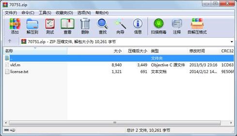
 属性            大小     日期    时间   名称
----------- ---------  ---------- -----  ----
     文件        8940  2013-05-03 15:16  vkf.m
     文件        1321  2014-02-12 14:24  license.txt